Demands

As TIAM-FR operates as a partial-equilibrium model, it requires a baseline energy service demand level for all energy services considered. Table 1 presents a comprehensive list of energy-service demands for every sector with their description, unit and time representation, i.e. either annually, seasonnaly, or hourly satisfied (Daynite). Each energy-service demand is associated with a specific driver (see last column of Table 1), facilitating the projection of future demand throughout the model horizon (2018 to 2100).

Table 1: Comprehensive list of energy and material demands in TIAM-FR

Demand	Description	Unit	TimeSlice	Driver
NEU	Non Energy Uses	PJ	Annual	GDPP
TAD	Domestic Aviation	PJ	Annual	POP
TAI	International Aviation	PJ	Annual	POP
TRB	Road Bus	Bv-km	Daynite	GDPP
TRC	Road Commercial Trucks	Bv-km	Daynite	GDPP
TRE	Road Three Wheels	Bv-km	Daynite	POP
TRH	Road Heavy Trucks	Bv-km	Daynite	GDPP
TRL	Road Light Vehicle	Bv-km	Daynite	GDPP
TRM	Road Medium Trucks	Bv-km	Daynite	GDPP
TRT	Road Auto	Bv-km	Daynite	GDPP
TRW	Road Two Wheels	Bv-km	Daynite	POP
TTF	Rail-Freight	PJ	Daynite	GDP
TTP	Rail-Passengers	PJ	Annual	POP
TWD	Domestic Internal Navigation	PJ	Annual	GDPP
TWI	International Navigation	PJ	Annual	GDPP
AGR	Agriculture Demand	PJ	Annual	GDPP
CSC	Commercial Space Cooling	PJ	Daynite	GDPP
CCK	Commercial Cooking	PJ	Daynite	GDPP
CSH	Commercial Space Heating	PJ	Season	GDPP
CHW	Commercial Hot Water	PJ	Daynite	GDPP
CLA	Commercial Lighting	PJ	Daynite	GDPP
COE	Commercial Office Equipment	PJ	Daynite	GDPP
CRF	Commercial Refrigeration	PJ	Daynite	GDPP
COT	Commercial Other	PJ	Daynite	GDPP
RSC	Residential Space Cooling	PJ	Daynite	HOU
RCD	Residential Clothes Drying	PJ	Daynite	HOU
RCW	Residential Clothes Washing	PJ	Daynite	HOU
RDW	Residential Dishwashing	PJ	Daynite	HOU
REA	Residential Other  Electric	PJ	Daynite	HOU
RSH	Residential Space Heating	PJ	Season	HOU
RHW	Residential Hot Water	PJ	Daynite	POP
RCK	Residential Cooking	PJ	Daynite	POP
RLI	Residential Lighting	PJ	Daynite	GDPP
RRF	Residential Refrigeration	PJ	Daynite	HOU
ROT	Residential Other	PJ	Daynite	HOU
ICH	Industry Chemicals	PJ	Annual	GDPP
IIS	Industry Iron & Steel	mt	Annual	GDPP
ILP	Industry Pulp & Paper	mt	Annual	GDPP
INF	Industry Non-Ferrous	mt	Annual	GDPP
INM	Industry Non-Metals	mt	Annual	GDPP
IOI	Industry Other Industry	PJ	Annual	GDPP
ICH_FS	Industry Chemicals Feedstocks	PJ	Annual	GDPP
ONO	Other Non-Specified Consumption	PJ	Annual	GDPP

These drivers are linked to the energy-service demands through a constant and an elasticity, following equation (1).

The demand drivers encompass population (POP), GDP, number of households (HOU), GDP per capita (GDPP) and GDP per household (GDPPHOU). The approach adopted in TIAM-FR consists of updating the energy and material demands from existing prospective studies from the International Institute for Applied System Analysis (IIASA), based on their Shared Socio-economic Pathways (SSP). Recently in the climate change research community, five narratives have been designed corresponding to different socio-economic and geopolitics pathways for the 21st century (Riahi et al., 2017, Dellinck, 2017). They explore how the world could tackle the challenges of climate change in terms of adaptation, impacts, vulnerabilities, and mitigation according to narrative’s description in terms of the evolution of inequalities, region rivalry, fossil-fueled development, and sustainable development. Each SSP has been studied by different laboratories to understand how to solve the climate problem according to their narrative. The IIASA SSP database (Riahi, 2017) is used to extract the final energy demand of industrial, transport, residential, and commercial sectors, according to:

• The region of the world, namely the OECD, Reforming Economies, Asia, Middle East and Africa, and Latin America,

• the SSP,

• the climate target based on radiative forcing constraints from 1.9 W/m² to 6.0 W/m², and also including a baseline with no climate constraint.

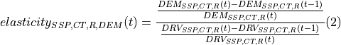
The socio-economic drivers are then used to calculate for each SSP, each region R, and each climate target CT, the elasticities of sector-specific energy demand DEM to their own drivers DRV over time t. We calculate the elasticities based on the following formula:

The sector-specific demands are divided into industry, residential and commercial sectors, and transportation, which is much more aggregated than in TIAM-FR, so we allocate each subsector of TIAM-FR to the right sector of IIASA database. Likewise, as the regions in the SSP database are much more aggregated than in TIAM-FR, the following allocation is done:

Table1: Region allocation between TIAM-FR and IIASA database

TIAM-FR	IIASA database
AFR	Middle East and Africa
AUS	OECD
CAN	OECD
CHI	Asia
CSA	Latin America
EEU	Reforming Economies
FSU	Reforming Economies
IND	Asia
JPN	OECD
MEA	Middle East and Africa
MEX	Latin America
ODA	Asia
SKO	OECD
USA	OECD
WEU	OECD

With elasticities estimated from equation (2), the demand are then calculated with equation (3):

References
Riahi, K., van Vuuren, D.P., Kriegler, E., Edmonds, J., O’Neill, B.C., Fujimori, S., Bauer, N., Calvin, K., Dellink, R., Fricko, O., Lutz, W., Popp, A., Cuaresma, J.C., Kc, S., Leimbach, M., Jiang, L., Kram, T., Rao, S., Emmerling, J., Ebi, K., Hasegawa, T., Havlik, P., Humpenöder, F., Da Silva, L.A., Smith, S., Stehfest, E., Bosetti, V., Eom, J., Gernaat, D., Masui, T., Rogelj, J., Strefler, J., Drouet, L., Krey, V., Luderer, G., Harmsen, M., Takahashi, K., Baumstark, L., Doelman, J.C., Kainuma, M., Klimont, Z., Marangoni, G., Lotze-Campen, H., Obersteiner, M., Tabeau, A., Tavoni, M., 2017. The Shared Socioeconomic Pathways and their energy, land use, and greenhouse gas emissions implications: An overview. Global Environmental Change 42, 153–168. https://doi.org/10.1016/j.gloenvcha.2016.05.009

Dellink, R., Chateau, J., Lanzi, E., Magné, B., 2017. Long-term economic growth projections in the Shared Socioeconomic Pathways. Global Environmental Change 42, 200–214. https://doi.org/10.1016/j.gloenvcha.2015.06.004